Introduction

In recent years, the field of computer vision has been revolutionized by the advent of transformer models. Originally designed for natural language processing tasks, transformers have proven to be incredibly powerful in capturing spatial dependencies in visual data as well. The Vision Transformer (ViT) is a prime example of this, presenting a novel architecture that achieves state-of-the-art performance on various image classification tasks.

In this article, we will embark on a journey to build our very own Vision Transformer using PyTorch. By breaking down the implementation step by step, we aim to provide a comprehensive understanding of the ViT architecture and enable you to grasp its inner workings with clarity. Of course, we could always use the PyTorch's inbuilt implementation of the Vision Transformer Model, but what's the fun in that.

We will start by setting up the necessary dependencies and libraries, ensuring a smooth workflow throughout the project. Next, we will dive into data acquisition, where we obtain a suitable dataset to train our Vision Transformer model.

To prepare the data for training, we will define the necessary transformations required for augmenting and normalizing the input images. With the data transformations in place, we will proceed to create a custom dataset and data loaders, setting the stage for training our model.

For understanding the Vision Transformer architecture, it is crucial to build it from scratch. In the subsequent sections, we will dissect each component of the ViT model and explain its purpose. We will begin with the Patch Embedding Layer, responsible for dividing the input image into smaller patches and embedding them into a vector format. Following that, we will explore the Multi-Head Self Attention Block, which allows the model to capture global and local relationships within the patches.

Additionally, we will delve into the Machine Learning Perceptron Block, a key component that enables the model to capture the hierarchical representations of the input data. By assembling these components, we will construct the Transformer Block, which forms the core building block of the Vision Transformer.

Finally, we will bring it all together by creating the ViT model, utilizing the components we have meticulously crafted. With the completed model, we can experiment with it, fine-tune it, and unleash its potential on various computer vision tasks.

By the end of this post, you will have gained a solid understanding of the Vision Transformer architecture and its implementation in PyTorch. Armed with this knowledge, you will be able to modify and extend the model to suit your specific needs or even build upon it for advanced computer vision applications. Let's start.

Step 0: Install and Import Dependencies

!pip install -q torchinfo

import torch
from torch import nn
from torchinfo import summary

Step 1: Get the Data

1.1. Download the Data from the Web (It will be a .zip file for this) 1.2. Extract the zip file 1.3. Delete the zip file

import requests
from pathlib import Path
import os
from zipfile import ZipFile

# Define the URL for the zip file
url = "https://github.com/mrdbourke/pytorch-deep-learning/raw/main/data/pizza_steak_sushi.zip"

# Send a GET request to download the file
response = requests.get(url)

# Define the path to the data directory
data_path = Path("data")

# Define the path to the image directory
image_path = data_path / "pizza_steak_sushi"

# Check if the image directory already exists
if image_path.is_dir():
    print(f"{image_path} directory exists.")
else:
    print(f"Did not find {image_path} directory, creating one...")
    image_path.mkdir(parents=True, exist_ok=True)

# Write the downloaded content to a zip file
with open(data_path / "pizza_steak_sushi.zip", "wb") as f:
    f.write(response.content)

# Extract the contents of the zip file to the image directory
with ZipFile(data_path / "pizza_steak_sushi.zip", "r") as zipref:
    zipref.extractall(image_path)

# Remove the downloaded zip file
os.remove(data_path / 'pizza_steak_sushi.zip')

Step 2: Define Transformations

Resize the images using Resize() to 224. We choose the images size to be 224 based on the ViT Paper
Convert to Tensor using ToTensor()

from torchvision.transforms import Resize, Compose, ToTensor

# Define the train_transform using Compose
train_transform = Compose([
    Resize((224, 224)),
    ToTensor()
])

# Define the test_transform using Compose
test_transform = Compose([
    Resize((224, 224)),
    ToTensor()
])

Step 3: Create Dataset and DataLoader

We can use PyTorch's ImageFolder DataSet library to create our Datasets.

For ImageFolder to work this is how your data folder needs to be structured.

data
└── pizza_steak_sushi
    ├── test
    │   ├── pizza
    │   ├── steak
    │   └── sushi
    └── train
        ├── pizza
        ├── steak
        └── sushi

All the pizza images will be in the pizza folder of train and test sub folders and so on for all the classes that you have.

There are two useful methods that you can call on the created training_dataset and test_dataset

training_dataset.classes that gives ['pizza', 'steak', 'sushi']
training_dataset.class_to_idx that gives {'pizza': 0, 'steak': 1, 'sushi': 2}

from torchvision.datasets import ImageFolder
from torch.utils.data import DataLoader

BATCH_SIZE = 32

# Define the data directory
data_dir = Path("data/pizza_steak_sushi")

# Create the training dataset using ImageFolder
training_dataset = ImageFolder(root=data_dir / "train", transform=train_transform)

# Create the test dataset using ImageFolder
test_dataset = ImageFolder(root=data_dir / "test", transform=test_transform)

# Create the training dataloader using DataLoader
training_dataloader = DataLoader(
    dataset=training_dataset,
    shuffle=True,
    batch_size=BATCH_SIZE,
    num_workers=2
)

# Create the test dataloader using DataLoader
test_dataloader = DataLoader(
    dataset=test_dataset,
    shuffle=False,
    batch_size=BATCH_SIZE,
    num_workers=2
)

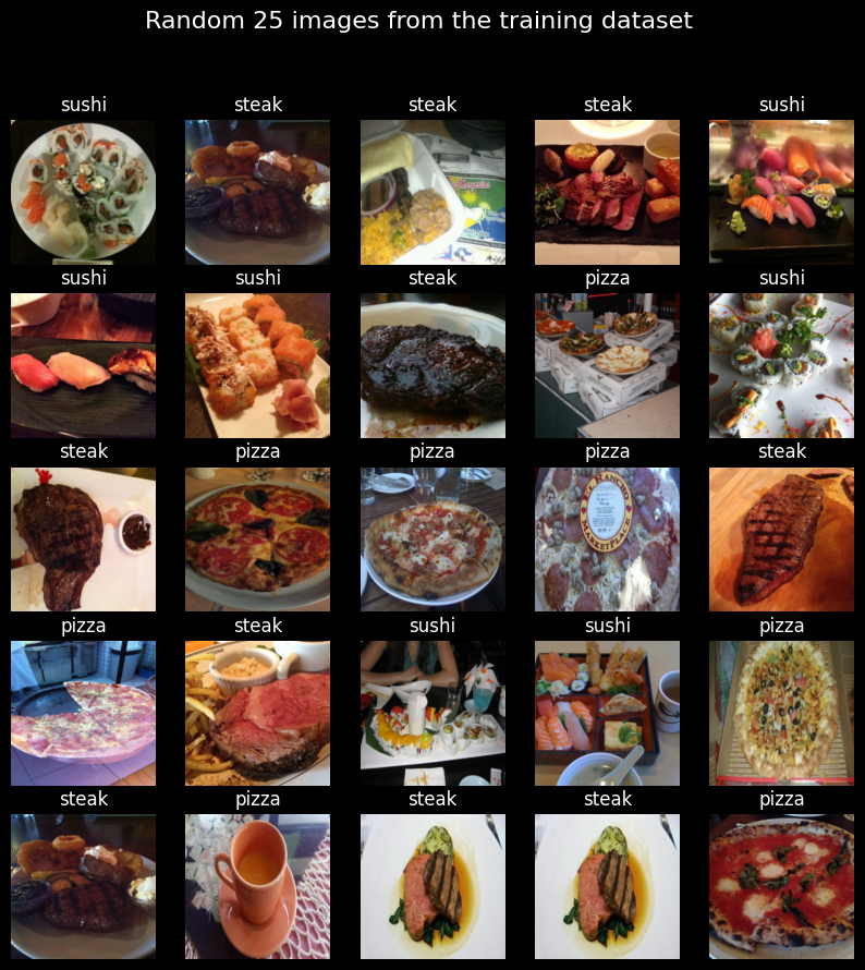
We can visualize a few training dataset images and see their labels

import matplotlib.pyplot as plt
import random

num_rows = 5
num_cols = num_rows

# Create a figure with subplots
fig, axs = plt.subplots(num_rows, num_cols, figsize=(10, 10))

# Iterate over the subplots and display random images from the training dataset
for i in range(num_rows):
    for j in range(num_cols):
        # Choose a random index from the training dataset
        image_index = random.randrange(len(training_dataset))

        # Display the image in the subplot
        axs[i, j].imshow(training_dataset[image_index][0].permute((1, 2, 0)))

        # Set the title of the subplot as the corresponding class name
        axs[i, j].set_title(training_dataset.classes[training_dataset[image_index][1]], color="white")

        # Disable the axis for better visualization
        axs[i, j].axis(False)

# Set the super title of the figure
fig.suptitle(f"Random {num_rows * num_cols} images from the training dataset", fontsize=16, color="white")

# Set the background color of the figure as black
fig.set_facecolor(color='black')

# Display the plot
plt.show()

dataset images

Understanding Vision Transformer Architecture

Let us take some time now to understand the Vision Transformer Architecture. This is the link to the original vision transformer paper: arxiv.org/abs/2010.11929.

Below, you can see the architecture that is proposed in the image.

The Vision Transformer (ViT) is a type of Transformer architecture designed for image processing tasks. Unlike traditional Transformers that operate on sequences of word embeddings, ViT operates on sequences of image embeddings. In other words, it breaks down an input image into patches and treats them as a sequence of learnable embeddings.

At a broad level, what ViT does is, it:

Creates Patch Embeddings
1. Takes an input image of a given size $ (H \times W \times C)$ -> (Height, Width, Channels)
2. Breaks it down into $N$ patches of a given size: $P$ --> PATCH_SIZE
3. Converts the patches into a sequence of learnable embeddings vectors: $E ∈ R^{(P^2C) \times D}$
4. Prepends a classification token embedding vector to the learnable embeddings vectors
5. Adds the position embeddings to the learnable embeddings: $E_{pos} \in R^{(N+1) \times D}$
6. Passes embeddings through Transformer Blocks:

The patch embeddings, along with the classification token, are passed through multiple Transformer blocks.
Each Transformer block consists of a MultiHead Self-Attention Block (MSA Block) and a Multi-Layer Perceptron Block (MLP Block).
Skip connections are established between the input to the Transformer block and the input to the MSA block, as well as between the input to the MLP block and the output of the MLP block. These skip connections help mitigate the vanishing gradient problem as more Transformer blocks are added.

Performs Classification:

The final output from the Transformer blocks is passed through an MLP block.
The classification token, which contains information about the input image's class, is used to make predictions.

We will dive into each of these steps in detail, starting with the crucial process of creating patch embeddings.

Step 4: Create Patch Embedding Layer

For the ViT paper, we need to perform the following functions on the image before passing it to the MultiHead Self-Attention Transformer Layer

Convert the image into patches of 16 x 16 size.
Embed each patch into 768 dimensions. So each patch becomes a [1 x 768] Vector. There will be $N = \frac{H \times W}{P^2}$ number of patches for each image. This results in an image that is of the shape [14 x 14 x 768]
Flatten the image along a single vector. This will give a [196 x 768] Matrix, which is our Image Embedding Sequence.
Prepend the Class Token Embeddings to the above output
Add the Position Embeddings to the Class Token and Image Embeddings.

Vision Tranformer Steps

PATCH_SIZE = 16
IMAGE_WIDTH = 224
IMAGE_HEIGHT = IMAGE_WIDTH
IMAGE_CHANNELS = 3
EMBEDDING_DIMS = IMAGE_CHANNELS * PATCH_SIZE**2
NUM_OF_PATCHES = int((IMAGE_WIDTH * IMAGE_HEIGHT) / PATCH_SIZE**2)

#the image width and image height should be divisible by patch size. This is a check to see that.

assert IMAGE_WIDTH % PATCH_SIZE == 0 and IMAGE_HEIGHT % PATCH_SIZE ==0 , print("Image Width is not divisible by patch size")

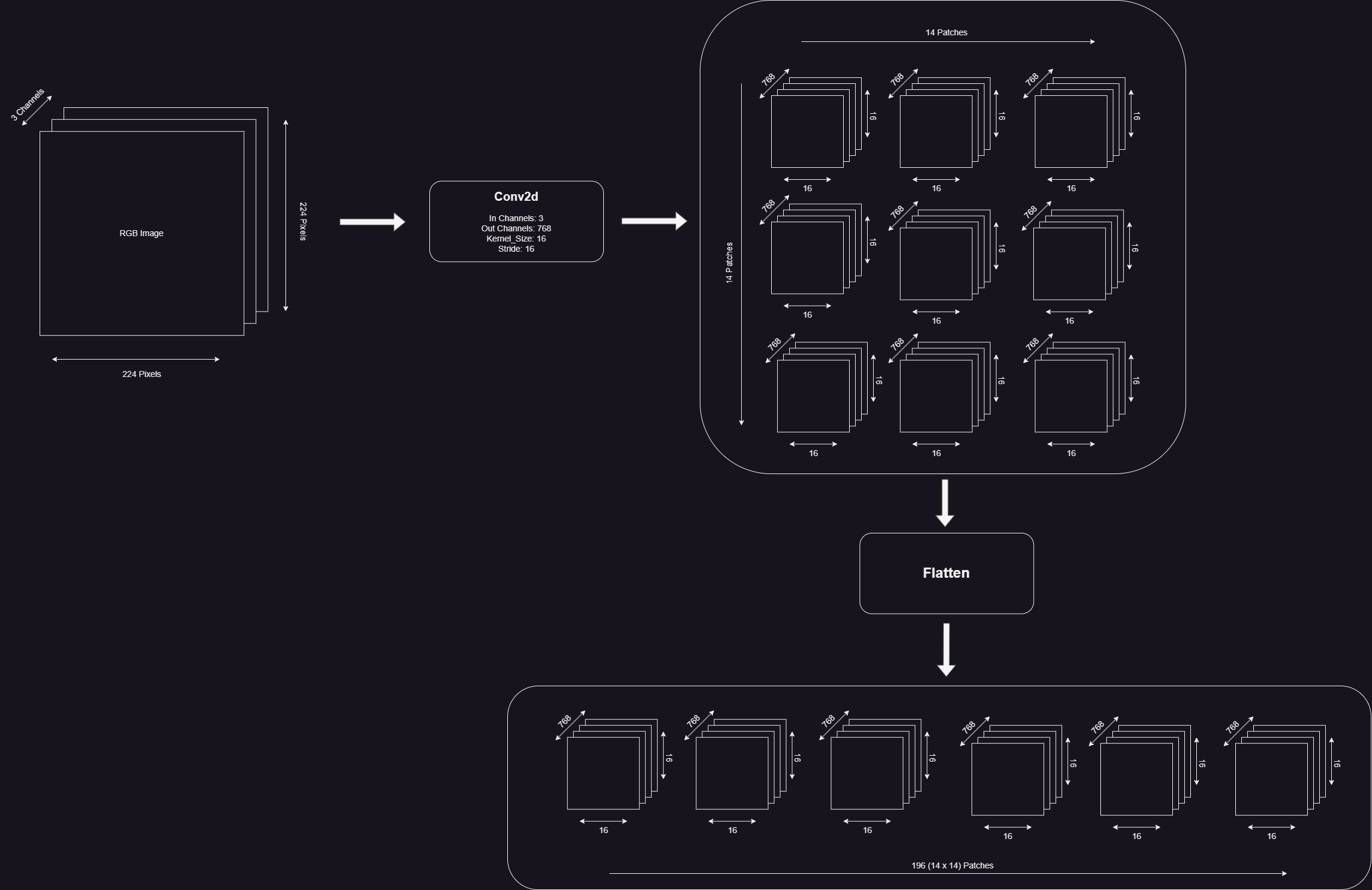
Step 4.1 Converting the image into patches of 16 x 16 and creating an embedding vector for each patch of size 768.

This can be accomplished by using a Conv2D Layer with a kernel_size equal to patch_size and a stride equal to patch_size

Convolution plus Flatten

conv_layer = nn.Conv2d(in_channels = IMAGE_CHANNELS, out_channels = EMBEDDING_DIMS, kernel_size = PATCH_SIZE, stride = PATCH_SIZE)

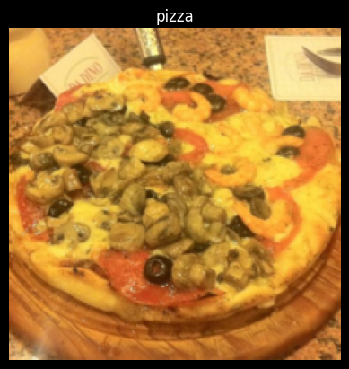
We can pass a random image into the convolutional layer and see what happens

random_images, random_labels = next(iter(training_dataloader))
random_image = random_images[0]

# Create a new figure
fig = plt.figure(1)

# Display the random image
plt.imshow(random_image.permute((1, 2, 0)))

# Disable the axis for better visualization
plt.axis(False)

# Set the title of the image
plt.title(training_dataset.classes[random_labels[0]], color="white")

# Set the background color of the figure as black
fig.set_facecolor(color="black")

random image

We need to change the shape to [1, 14, 14, 768] and flatten the output to [1, 196, 768]

# Pass the image through the convolution layer
image_through_conv = conv_layer(random_image.unsqueeze(0))
print(f'Shape of embeddings through the conv layer -> {list(image_through_conv.shape)} <- [batch_size, num_of_patch_rows,num_patch_cols embedding_dims]')

# Permute the dimensions of image_through_conv to match the expected shape
image_through_conv = image_through_conv.permute((0, 2, 3, 1))

# Create a flatten layer using nn.Flatten
flatten_layer = nn.Flatten(start_dim=1, end_dim=2)

# Pass the image_through_conv through the flatten layer
image_through_conv_and_flatten = flatten_layer(image_through_conv)

# Print the shape of the embedded image
print(f'Shape of embeddings through the flatten layer -> {list(image_through_conv_and_flatten.shape)} <- [batch_size, num_of_patches, embedding_dims]')

# Assign the embedded image to a variable
embedded_image = image_through_conv_and_flatten

Shape of embeddings through the conv layer -> [1, 768, 14, 14] <- [batch_size, num_of_patch_rows,num_patch_cols embedding_dims]
Shape of embeddings through the flatten layer -> [1, 196, 768] <- [batch_size, num_of_patches, embedding_dims]

4.2. Prepending the Class Token Embedding and Adding the Position Embeddings

class_token_embeddings = nn.Parameter(torch.rand((1, 1,EMBEDDING_DIMS), requires_grad  = True))
print(f'Shape of class_token_embeddings --> {list(class_token_embeddings.shape)} <-- [batch_size, 1, emdedding_dims]')

embedded_image_with_class_token_embeddings = torch.cat((class_token_embeddings, embedded_image), dim = 1)
print(f'\nShape of image embeddings with class_token_embeddings --> {list(embedded_image_with_class_token_embeddings.shape)} <-- [batch_size, num_of_patches+1, embeddiing_dims]')

position_embeddings = nn.Parameter(torch.rand((1, NUM_OF_PATCHES+1, EMBEDDING_DIMS ), requires_grad = True ))
print(f'\nShape of position_embeddings --> {list(position_embeddings.shape)} <-- [batch_size, num_patches+1, embeddings_dims]')

final_embeddings = embedded_image_with_class_token_embeddings + position_embeddings
print(f'\nShape of final_embeddings --> {list(final_embeddings.shape)} <-- [batch_size, num_patches+1, embeddings_dims]')

Shape of `class_token_embeddings` --> `[1, 1, 768]` <-- `[batch_size, 1, emdedding_dims]`

Shape of `image embeddings with class_token_embeddings` --> `[1, 197, 768]` <-- `[batch_size, num_of_patches+1, embeddiing_dims]`

Shape of `position_embeddings` --> `[1, 197, 768]` <-- `[batch_size, num_patches+1, embeddings_dims]`

Shape of `final_embeddings` --> `[1, 197, 768]` <-- `[batch_size, num_patches+1, embeddings_dims]`

Put the PatchEmbedddingLayer Together

We will inherit from the PyTorch nn.Module to create our custom layer which takes in an image and throws out the patch embeddings which consists of the Image Embeddings, Class Token Embeddings and the Position Embeddings.

class PatchEmbeddingLayer(nn.Module):
    def __init__(self, in_channels, patch_size, embedding_dim,):
        super().__init__()
        self.patch_size = patch_size
        self.embedding_dim = embedding_dim
        self.in_channels = in_channels
        self.conv_layer = nn.Conv2d(in_channels=in_channels, out_channels=embedding_dim, kernel_size=patch_size, stride=patch_size)
        self.flatten_layer = nn.Flatten(start_dim=1, end_dim=2)
        self.class_token_embeddings = nn.Parameter(torch.rand((BATCH_SIZE, 1, EMBEDDING_DIMS), requires_grad=True))
        self.position_embeddings = nn.Parameter(torch.rand((1, NUM_OF_PATCHES + 1, EMBEDDING_DIMS), requires_grad=True))

    def forward(self, x):
        output = torch.cat((self.class_token_embeddings, self.flatten_layer(self.conv_layer(x).permute((0, 2, 3, 1)))), dim=1) + self.position_embeddings
        return output

Let's pass a batch of random images from our patch embedding layer.

patch_embedding_layer = PatchEmbeddingLayer(in_channels=IMAGE_CHANNELS, patch_size=PATCH_SIZE, embedding_dim=IMAGE_CHANNELS * PATCH_SIZE ** 2)

patch_embeddings = patch_embedding_layer(random_images)
patch_embeddings.shape

torch.Size([32, 197, 768])

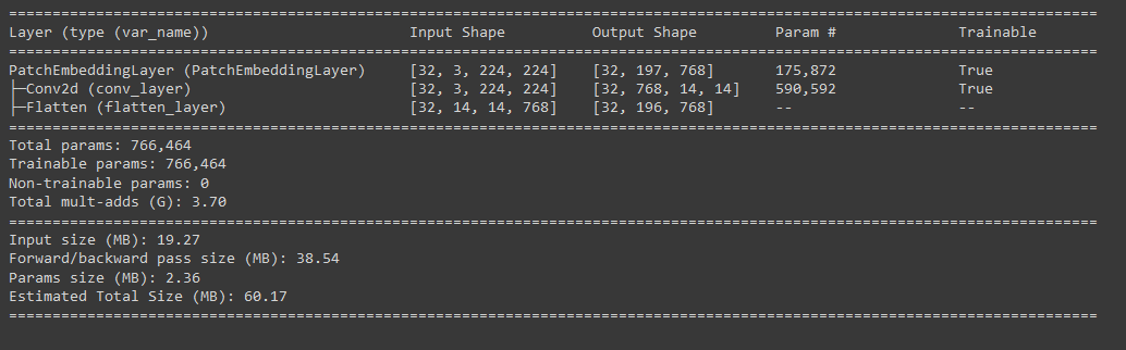
summary(model=patch_embedding_layer,
        input_size=(BATCH_SIZE, 3, 224, 224), # (batch_size, input_channels, img_width, img_height)
        col_names=["input_size", "output_size", "num_params", "trainable"],
        col_width=20,
        row_settings=["var_names"])

Patch Embedding

Step 5. Creating the Multi-Head Self Attention (MSA) Block.

Understanding MSA Block

As a first step of putting together our transformer block for the Vision Transformer model, we will be creating a MultiHead Self Attention Block.

Let us take a moment to understand the MSA Block. The MSA block itself consists of a LayerNorm layer and the Multi-Head Attention Layer. The layernorm layer essentially normalizes our patch embeddings data across the embeddings dimension. The Multi-Head Attention layer takes in the input data as 3 form of learnable vectors namely query, key and value, collectively known as qkv vectors. These vectors together form the relationship between each patch of the input sequence with every other patch in the same sequence (hence the name self-attention).

So, our input shape to the MSA Block will be the shape of our patch embeddings that we made using the PatchEmbeddingLayer -> [batch_size, sequence_length, embedding_dimensions]. And the output from the MSA layer will be of the same shape as the input.

MSA Block Code

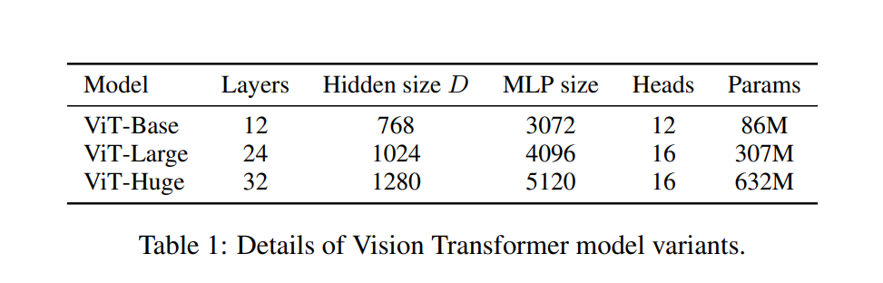
Now let us begin to write code for out MSA Block. This will be short as PyTorch has a pre-built implementation of LayerNorm and the MultiHeadAttention Layer. We just have to pass the right arguments to suit our architecture. We can find the various parameters that are required for out MSA block in this table from the original ViT Paper.

class MultiHeadSelfAttentionBlock(nn.Module):
  def __init__(self,
               embedding_dims = 768, # Hidden Size D in the ViT Paper Table 1
               num_heads = 12,  # Heads in the ViT Paper Table 1
               attn_dropout = 0.0 # Default to Zero as there is no dropout for the the MSA Block as per the ViT Paper
               ):
    super().__init__()

    self.embedding_dims = embedding_dims
    self.num_head = num_heads
    self.attn_dropout = attn_dropout

    self.layernorm = nn.LayerNorm(normalized_shape = embedding_dims)

    self.multiheadattention =  nn.MultiheadAttention(num_heads = num_heads,
                                                     embed_dim = embedding_dims,
                                                     dropout = attn_dropout,
                                                     batch_first = True,
                                                    )

  def forward(self, x):
    x = self.layernorm(x)
    output,_ = self.multiheadattention(query=x, key=x, value=x,need_weights=False)
    return output

Let's test our MSA Block

multihead_self_attention_block = MultiHeadSelfAttentionBlock(embedding_dims = EMBEDDING_DIMS,
                                                             num_heads = 12
                                                             )
print(f'Shape of the input Patch Embeddings => {list(patch_embeddings.shape)} <= [batch_size, num_patches+1, embedding_dims ]')
print(f'Shape of the output from MSA Block => {list(multihead_self_attention_block(patch_embeddings).shape)} <= [batch_size, num_patches+1, embedding_dims ]')

Shape of the input Patch Embeddings => [32, 197, 768] <= [batch_size, num_patches+1, embedding_dims ] Shape of the output from MSA Block => [32, 197, 768] <= [batch_size, num_patches+1, embedding_dims ]

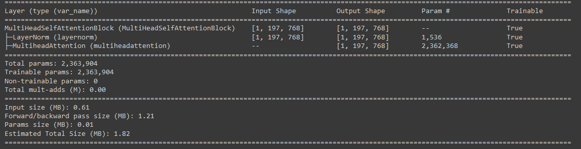
Beautiful, so seems like our MSA block is working. We can get more information about the MSA Block using torchinfo

summary(model=multihead_self_attention_block,
        input_size=(1, 197, 768), # (batch_size, num_patches, embedding_dimension)
        col_names=["input_size", "output_size", "num_params", "trainable"],
        col_width=20,
        row_settings=["var_names"])

MSA_Block

Step 6. Creating the Machine Learning Perceptron (MLP) Block

Understanding the MLP Block

The Machine Learning Perceptron (MLP) Block in the transformer is a combination of a Fully Connected Layer (also called as a Linear Layer or a Dense Layer) and a non-linear layer. In the case of ViT, the non-linear layer is a GeLU layer.

The transformer also implements a Dropout layer to reduce overfitting. So the MLP Block will look something like this:

Input → Linear → GeLU → Dropout → Linear → Dropout

According to the paper, the first Linear Layer scales the embedding dimensions to the 3072 dimensions (for the ViT-16/Base). The Dropout is set to 0.1 and the second Linear Layer scales down the dimensions back to the embedding dimensions.

MLP Block Code

Let us now assemble our MLP Block. According to the ViT Paper, the output from the MSA Block added to the input to the MSA Block (denoted by the skip/residual connection in the model architecture figure) is passed as input to the MLP Block. All the layers are provided by the PyTorch library. We just need to assemble it.

class MachineLearningPerceptronBlock(nn.Module):
  def __init__(self, embedding_dims, mlp_size, mlp_dropout):
    super().__init__()
    self.embedding_dims = embedding_dims
    self.mlp_size = mlp_size
    self.dropout = mlp_dropout

    self.layernorm = nn.LayerNorm(normalized_shape = embedding_dims)
    self.mlp = nn.Sequential(
        nn.Linear(in_features = embedding_dims, out_features = mlp_size),
        nn.GELU(),
        nn.Dropout(p = mlp_dropout),
        nn.Linear(in_features = mlp_size, out_features = embedding_dims),
        nn.Dropout(p = mlp_dropout)
    )

  def forward(self, x):
    return self.mlp(self.layernorm(x))

Let's test our MLP Block

mlp_block = MachineLearningPerceptronBlock(embedding_dims = EMBEDDING_DIMS,
                                           mlp_size = 3072,
                                           mlp_dropout = 0.1)

summary(model=mlp_block,
        input_size=(1, 197, 768), # (batch_size, num_patches, embedding_dimension)
        col_names=["input_size", "output_size", "num_params", "trainable"],
        col_width=20,
        row_settings=["var_names"])

MLP_Block

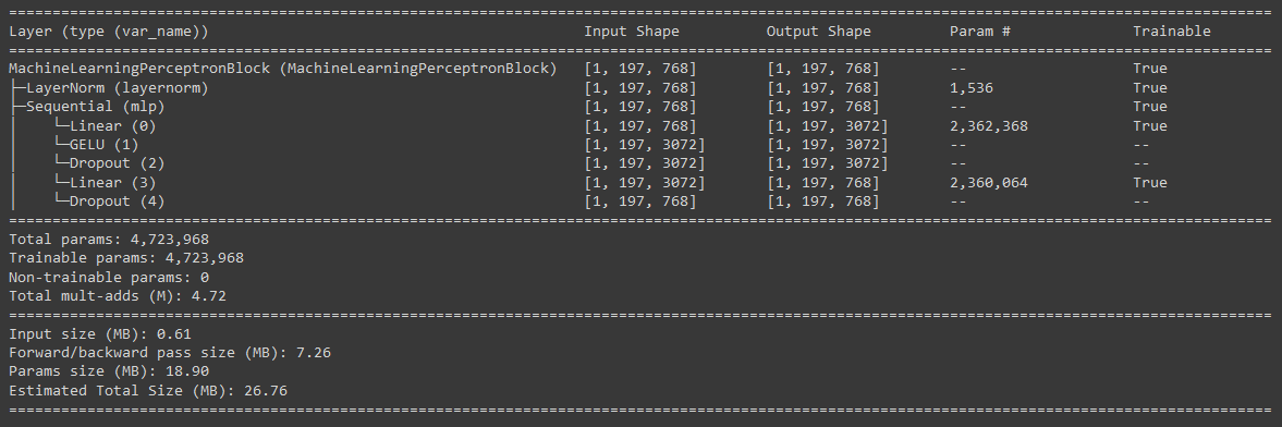
Amazing, looks like the MLP Block is also working as expected.

Step 7. Putting together the Transformer Block

class TransformerBlock(nn.Module):
  def __init__(self, embedding_dims = 768,
               mlp_dropout=0.1,
               attn_dropout=0.0,
               mlp_size = 3072,
               num_heads = 12,
               ):
    super().__init__()

    self.msa_block = MultiHeadSelfAttentionBlock(embedding_dims = embedding_dims,
                                                 num_heads = num_heads,
                                                 attn_dropout = attn_dropout)

    self.mlp_block = MachineLearningPerceptronBlock(embedding_dims = embedding_dims,
                                                    mlp_size = mlp_size,
                                                    mlp_dropout = mlp_dropout,
                                                    )

  def forward(self,x):
    x = self.msa_block(x) + x
    x = self.mlp_block(x) + x

    return x

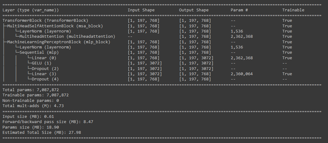
Testing the Transformer Block

transformer_block = TransformerBlock(embedding_dims = EMBEDDING_DIMS,
                                     mlp_dropout = 0.1,
                                     attn_dropout=0.0,
                                     mlp_size = 3072,
                                     num_heads = 12)

print(f'Shape of the input Patch Embeddings => {list(patch_embeddings.shape)} <= [batch_size, num_patches+1, embedding_dims ]')
print(f'Shape of the output from Transformer Block => {list(transformer_block(patch_embeddings).shape)} <= [batch_size, num_patches+1, embedding_dims ]')

Shape of the input Patch Embeddings => [32, 197, 768] <= [batch_size, num_patches+1, embedding_dims ]
Shape of the output from Transformer Block => [32, 197, 768] <= [batch_size, num_patches+1, embedding_dims ]

summary(model=transformer_block,
        input_size=(1, 197, 768), # (batch_size, num_patches, embedding_dimension)
        col_names=["input_size", "output_size", "num_params", "trainable"],
        col_width=20,
        row_settings=["var_names"])

Transformer Block

Step 8. Creating the ViT Model

Finally, let’s put together our ViT Model. It’s going to be as simple as combining whatever we have done till now. One slight addition will be the classifier layer that we will add. In ViT the classifier layer is a simple Linear layer with Layer Normalization. The classification is performed on the zeroth index of the output of the transformer.

class ViT(nn.Module):
  def __init__(self, img_size = 224,
               in_channels = 3,
               patch_size = 16,
               embedding_dims = 768,
               num_transformer_layers = 12, # from table 1 above
               mlp_dropout = 0.1,
               attn_dropout = 0.0,
               mlp_size = 3072,
               num_heads = 12,
               num_classes = 1000):
    super().__init__()

    self.patch_embedding_layer = PatchEmbeddingLayer(in_channels = in_channels,
                                                     patch_size=patch_size,
                                                     embedding_dim = embedding_dims)

    self.transformer_encoder = nn.Sequential(*[TransformerBlock(embedding_dims = embedding_dims,
                                              mlp_dropout = mlp_dropout,
                                              attn_dropout = attn_dropout,
                                              mlp_size = mlp_size,
                                              num_heads = num_heads) for _ in range(num_transformer_layers)])

    self.classifier = nn.Sequential(nn.LayerNorm(normalized_shape = embedding_dims),
                                    nn.Linear(in_features = embedding_dims,
                                              out_features = num_classes))

  def forward(self, x):
    return self.classifier(self.transformer_encoder(self.patch_embedding_layer(x))[:, 0])

summary(model=vit,
        input_size=(BATCH_SIZE, 3, 224, 224), # (batch_size, num_patches, embedding_dimension)
        col_names=["input_size", "output_size", "num_params", "trainable"],
        col_width=20,
        row_settings=["var_names"])

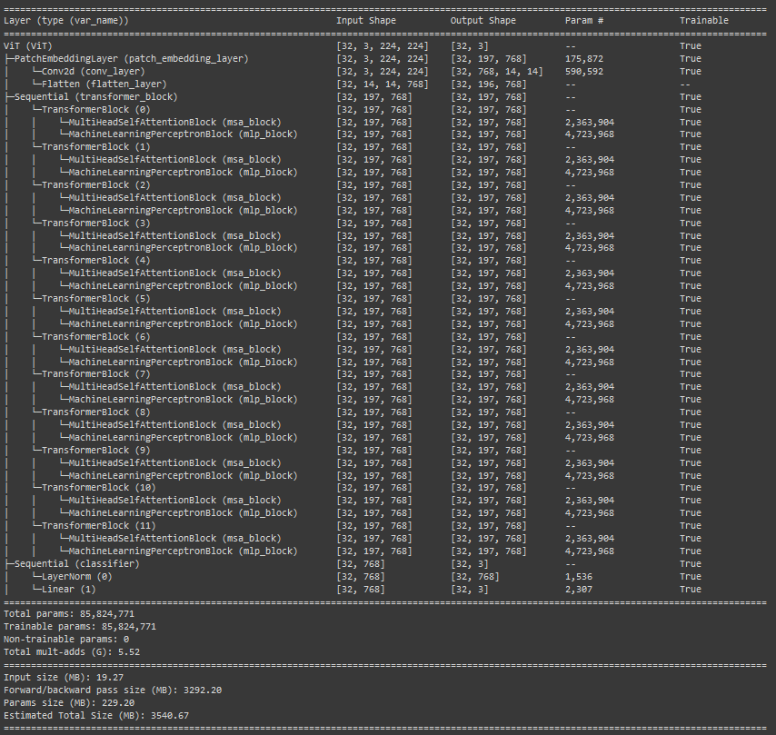
That's it. Now you can train this model just like you would any other model in PyTorch. Let me know how it works out for you.

That’s it. Now you can train this model just like you would any other model in PyTorch. Let me know how it works out for you. I hope this step-by-step guide has helped you understand the Vision Transformer and inspired you to dive deeper into the world of computer vision and transformer models. With the knowledge gained, you are well-equipped to push the boundaries of computer vision and unlock the potential of these groundbreaking architectures.

So go ahead, build upon what you have learned, and let your imagination run wild as you leverage the Vision Transformer to tackle exciting visual challenges. Happy coding!

Akshay's Blog