In the previous part of our blog series, we discussed how to initialize a neural network (NN) model with specified layers and hidden units. Now, in this part, we will explore the forward propagation algorithm, a fundamental step in the NN's prediction process.
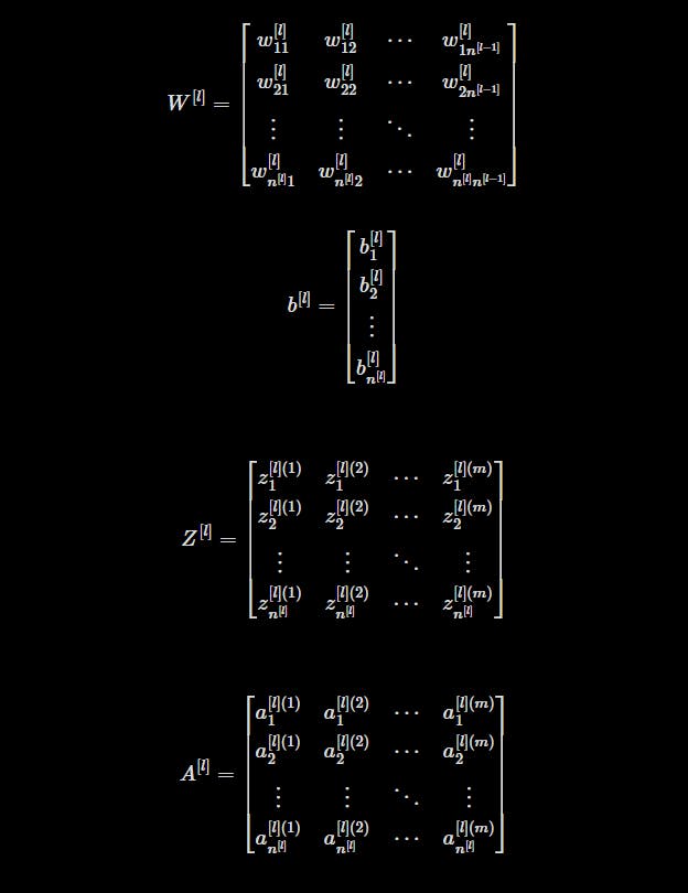
Before we delve into the coding aspect, let's understand the mathematical concepts underlying forward propagation. We will use the following notations:
Z[l]: Logit Matrix for layer
l. It represents the linear transformation of the inputs for a particular layer.A[l]: Activation matrix for layer
l. It represents the output or activation values of the neurons in a specific layer.W[l]: Weights matrix for layer
l. It contains the weights connecting the neurons of layerl-1to the neurons of layerl.b[l]: Bias matrix for layer
l. It contains the bias values added to the linear transformation of the inputs for layerl.
Additionally, we have the input matrix denoted as X, which is equal to the activation matrix A[0] of the input layer.
To perform forward propagation, we need to follow these two steps for each layer:
1. Calculate the logit matrix for each layer using the following expression:
Z[l] = W[l]A[l-1] + b[l]
In simpler terms, the logit matrix for layer l is obtained by taking the dot product of the weight matrix W[l] and the activation matrix A[l-1] from the previous layer, and then adding the bias matrix b[l]. This step represents the linear transformation of the inputs for the current layer.
2. Calculate the activation matrix from the logit matrix using an activation function:
A[l] = ActivationFunction(Z[l])
Here, the activation function can be any non-linear function applied element-wise to the elements of the logit matrix. Popular activation functions include sigmoid, tanh, and relu. In our model, we will use the relu activation function for all intermediate layers and sigmoid for the last layer (classifier layer). This step introduces non-linearity into the network, allowing it to learn and model complex relationships in the data.
For n[l] number of hidden units in layer l and m number of examples, these are the shapes of each matrix:
Z[l] ⇾ [n[l] x m]
W[l] ⇾ [n[l] x n[l-1]]
b[l] ⇾ [n[l] x 1]
A[l] ⇾ [n[l] x m]

During the forward propagation process, we will store the weight matrix, bias matrix, and logit matrix as cache. This stored information will prove useful in the subsequent step of backward propagation, where we update the model's parameters based on the computed gradients.
By performing forward propagation, our neural network takes the input data through all the layers, applying linear transformations and activation functions, and eventually produces a prediction or output at the final layer.
Dependencies
Add this line to the Cargo.toml file.
num-integer = "0.1.45"
Cache Structs
First, in the lib.rs file we will define two structs - LinearCache and ActivationCache
//lib.rs

use num_integer::Roots;

#[derive(Clone, Debug)]
pub struct LinearCache {
    pub a: Array2<f32>,
    pub w: Array2<f32>,
    pub b: Array2<f32>,
}

#[derive(Clone, Debug)]
pub struct ActivationCache {
    pub z: Array2<f32>,
}
The LinearCache struct stores the intermediate values needed for each layer. It includes the activation matrix a, weight matrix w, and bias matrix b. These matrices are used to calculate the logit matrix z in the forward propagation process.
The ActivationCache struct stores the logit matrix z for each layer. This cache is essential for later stages, such as backpropagation, where the stored values are required.
Define Activation Functions
Next, let us define the non-linear activation functions that we will be using - relu and sigmoid
//lib.rs

pub fn sigmoid(z: &f32) -> f32 {
    1.0 / (1.0 + E.powf(-z))
}

pub fn relu(z: &f32) -> f32 {
    match *z > 0.0 {
        true => *z,
        false => 0.0,
    }
}

pub fn sigmoid_activation(z: Array2<f32>) -> (Array2<f32>, ActivationCache) {
    (z.mapv(|x| sigmoid(&x)), ActivationCache { z })
}

pub fn relu_activation(z: Array2<f32>) -> (Array2<f32>, ActivationCache) {
    (z.mapv(|x| relu(&x)), ActivationCache { z })
}
Activation functions introduce non-linearity to neural networks and play a crucial role in the forward propagation process. The code provides implementations for two commonly used activation functions: sigmoid and relu.
The sigmoid function takes a single value z as input and returns the sigmoid activation, which is calculated using the sigmoid formula: 1 / (1 + e^-z). The sigmoid function maps the input value to a range between 0 and 1, enabling the network to model non-linear relationships.
The relu function takes a single value z as input and applies the Rectified Linear Unit (ReLU) activation. If z is greater than zero, the function returns z; otherwise, it returns zero. ReLU is a popular activation function that introduces non-linearity and helps the network learn complex patterns.
Both sigmoid and relu functions are used for individual values or as building blocks for the matrix-based activation functions.
The code also provides two matrix-based activation functions: sigmoid_activation and relu_activation. These functions take a 2D matrix z as input and apply the respective activation function element-wise using the mapv function. The resulting activation matrix is returned along with an ActivationCache struct that stores the corresponding logit matrix.
Linear Forward
//lib.rs

pub fn linear_forward(
    a: &Array2<f32>,
    w: &Array2<f32>,
    b: &Array2<f32>,
) -> (Array2<f32>, LinearCache) {
    let z = w.dot(a) + b;

    let cache = LinearCache {
        a: a.clone(),
        w: w.clone(),
        b: b.clone(),
    };
    return (z, cache);
}
The linear_forward function takes the activation matrix a, weight matrix w, and bias matrix b as inputs. It performs the linear transformation by calculating the dot product of w and a, and then adding b to the result. The resulting matrix z represents the logits of the layer. The function returns z along with a LinearCache struct that stores the input matrices for later use in backward propagation.
Linear Forward Activation
//lib.rs

pub fn linear_forward_activation(
    a: &Array2<f32>,
    w: &Array2<f32>,
    b: &Array2<f32>,
    activation: &str,
) -> Result<(Array2<f32>, (LinearCache, ActivationCache)), String> {
    match activation {
        "sigmoid" => {
            let (z, linear_cache) = linear_forward(a, w, b);
            let (a_next, activation_cache) = sigmoid_activation(z);
            return Ok((a_next, (linear_cache, activation_cache)));
        }
        "relu" => {
            let (z, linear_cache) = linear_forward(a, w, b);
            let (a_next, activation_cache) = relu_activation(z);
            return Ok((a_next, (linear_cache, activation_cache)));
        }
        _ => return Err("wrong activation string".to_string()),
    }
}
The linear_forward_activation function builds upon the linear_forward function. It takes the same input matrices as linear_forward, along with an additional activation parameter indicating the activation function to be applied. The function first calls linear_forward to obtain the logits z and the linear cache. Then, depending on the specified activation function, it calls either sigmoid_activation or relu_activation to compute the activation matrix a_next and the activation cache. The function returns a_next along with a tuple of the linear cache and activation cache, wrapped in a Result enum. If the specified activation function is not supported, an error message is returned.
Forward Propagation
impl DeepNeuralNetwork {
/// Initializes the parameters of the neural network.
///
/// ### Returns
/// a Hashmap dictionary of randomly initialized weights and biases.
pub fn initialize_parameters(&self) -> HashMap<String, Array2<f32>> {
// same as last part
}
pub fn forward(
&self,
x: &Array2<f32>,
parameters: &HashMap<String, Array2<f32>>,
) -> (Array2<f32>, HashMap<String, (LinearCache, ActivationCache)>) {
let number_of_layers = self.layers.len()-1;
let mut a = x.clone();
let mut caches = HashMap::new();
for l in 1..number_of_layers {
let w_string = ["W", &l.to_string()].join("").to_string();
let b_string = ["b", &l.to_string()].join("").to_string();
let w = ¶meters[&w_string];
let b = ¶meters[&b_string];
let (a_temp, cache_temp) = linear_forward_activation(&a, w, b, "relu").unwrap();
a = a_temp;
caches.insert(l.to_string(), cache_temp);
}
// Compute activation of last layer with sigmoid
let weight_string = ["W", &(number_of_layers).to_string()].join("").to_string();
let bias_string = ["b", &(number_of_layers).to_string()].join("").to_string();
let w = ¶meters[&weight_string];
let b = ¶meters[&bias_string];
let (al, cache) = linear_forward_activation(&a, w, b, "sigmoid").unwrap();
caches.insert(number_of_layers.to_string(), cache);
return (al, caches);
}
}
The forward method in the DeepNeuralNetwork implementation performs the forward propagation process for the entire neural network. It takes the input matrix x and the parameters (weights and biases) as inputs. The method initializes the a matrix as a copy of x and creates an empty hashmap caches to store the caches for each layer.
Next, it iterates over each layer (except the last layer) in a for loop. For each layer, it retrieves the corresponding weights w and biases b from the parameters using string concatenation. It then calls linear_forward_activation with a, w, b, and the activation function set to "relu". The resulting activation matrix a_temp and the cache cache_temp are stored in the caches hashmap using the layer index as the key. The a matrix is updated to a_temp for the next iteration.
After processing all intermediate layers, the activation of the last layer is computed using the sigmoid activation function. It retrieves the weights w and biases b for the last layer from the parameters and calls linear_forward_activation with a, w, b, and the activation function set to "sigmoid". The resulting activation matrix al and the cache cache are stored in the caches hashmap using the last layer index as the key.
Finally, the method returns the final activation matrix al and the caches hashmap containing all the caches for each layer. Here al is the activation of the final layer and will be used to make the predictions during the inference part of our process.
That is all for Forward Propagation
In conclusion, we've covered an important aspect of building a deep neural network in this blog post: forward propagation. We learned how the input data moves through the layers, undergoes linear transformations, and is activated using different functions.
But our journey doesn't end here! In the next blog post, we'll dive into exciting topics like loss function and backward propagation. We'll explore how to measure the error between predictions and actual outputs, and how to use that error to update our model. These steps are crucial for training the neural network and improving its performance.
So, stay tuned for the next blog post, where we'll understand and implement a binary cross-entropy loss function and perform backpropagation.
🌐 My Website 🐦 Twitter 👨💼 LinkedIn
