Maze Solving Robot with Reinforcement Learning - Part 1
Basics and Theory for Reinforcement Learning

Machine Learning Enthusiast🤖 | AI Writer ✍️ | Rustacean🦀 | Entrepreneur 🚀| Cyclist 🚴
Exploring the endless possibilities of ML & AI. Sharing insights through engaging articles. Crafting robust solutions with Rust. Entrepreneurial mindset. Pedaling towards an innovative future! 🌟🔬🌳
Introduction to Reinforcement Learning
Hello everyone! Today, we are going to dive into the exciting world of Reinforcement Learning (RL). While RL has proven to be useful in various applications, it often gets overshadowed by the popularity of supervised and unsupervised learning. To demonstrate the power of RL, we will create an algorithm to solve complex mazes and visualize the results using Pygame. Think of this project as a Hello World for reinforcement learning!
In this Part 1, we will go over some basics and theory of Reinforcement Learning. If you want to skip to the code, you can head over to Part 2.
Agent - Environment Interaction
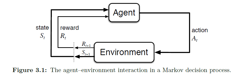
In Reinforcement Learning, we have an Agent that interacts with an Environment. The agent takes Actions (At) while being in a specific State (St). These actions lead the agent to a new state and result in a Reward (Rt) at a certain time step, denoted by t. This process continues until the agent reaches a final state, known as the Terminal State ST, or it continues indefinitely. If there is a terminal state, each agent's run is called an Episode. On the other hand, if the agent can perform actions indefinitely, it's known as a Continuing Task.
Let's define some of these terms more clearly:
State (St)
The state represents the current situation of the task environment. It contains all the relevant information needed to describe where the agent is in the environment at a specific time.
For example:
In a game of chess, the state includes the current positions of all the pieces on the board.
For a robotic arm, the state comprises the current rotations of each joint and the position of the end effector.
In a Pacman game, the state includes the position of the player, the position of the edibles, and the position of the ghosts.
Remember, the state is specific to a particular time t.
Action (At)
Actions are the choices the agent can make at a given time to influence the task or environment.
For example:
For a robotic arm, an action could involve adjusting the rotation of each arm to complete a task.
In a Pacman game, actions involve the buttons pressed by the player at a given moment.
The agent selects actions based on the current state of the environment.
Reward (Rt)
The reward is a numerical value that the agent receives upon performing an action. It represents the effectiveness or quality of the action taken.
For example:
In the case of a robotic arm, the agent might receive a reward of zero until it successfully completes the task. Once the task is completed, it receives a positive reward value.
In the Pacman game, the player is rewarded positively for eating a pill.
So, the agent's goal in reinforcement learning is to find a strategy (policy) that maximizes the total reward it receives over time.
Now the question is how do we formulize all of this in a framework and how are we supposed to know what actions lead to the highest accumulated reward in the long run. This is where Markov Decision Process comes in.
Markov Decision Process
Markov Decision Process (MDP) is a powerful mathematical framework used in Reinforcement Learning to model decision-making problems in environments that exhibit the Markov property. It provides a formal way to represent decision-making situations where the outcome of an action is uncertain and depends on the current state of the environment.
Now, what is a Markov Property.
Think of Reinforcement Learning (RL) as a way for a computer program to learn how to play a game. In this game, the computer, which we'll call the "agent," needs to make decisions to win or get rewards. The game world, where the agent plays, is called the "environment.". In this game, the agent can take different actions, like moving left, right, up, or down. Each action might lead to different outcomes or results, and the agent doesn't always know what will happen next. So, there's some uncertainty involved. Now, the interesting part is that the outcome of an action depends only on what's happening in the game right now. It doesn't matter how the game got to this point; all that matters is the current situation. This idea is called the "Markov property".
Let's get into a little bit of math. Shall we? If you don't like math, feel free to dive into the code. I have made sure to explain all this math more practically in the code section.
The Reward Hypothesis
At each time step, the agent receives a reward which is a simple scalar value and can be zero. The agent's goal in RL is to nothing but maximize the total amount of reward that it achieves in a run. Academically, reward hypothesis is defined as:
\>all of what we mean by goals and purposes can be well thought of as the maximization of the expected value of the cumulative sum of a received scalar signal (called reward).
For example, In making a robot learn how to escape from a maze, the reward is often -1 for every time step that passes prior to escape; this encourages the agent to escape as quickly as possible. We call this total reward that the agent receives as Return (Gt) Return and the Discounting Factor
In Reinforcement Learning, the agent's ultimate goal is to maximize the total amount of reward it receives during a run. This cumulative sum of received rewards is known as the Return and is denoted by Gt. To better understand this, let's think of it as follows:
At each time step t, the agent receives a reward, which is a simple scalar value, and it can be zero. The agent's task is to find a strategy that allows it to accumulate the highest possible reward over time. This idea is captured by the reward hypothesis, which says that all the goals and purposes of the agent can be thought of as maximizing the expected value of the cumulative sum of these rewards.
For example, let's consider the scenario of teaching a robot to escape from a maze. The agent might receive a reward of -1 for every time step that passes before it successfully escapes. This negative reward encourages the agent to find a path and escape as quickly as possible. We call this total reward that the agent receives as Return (Gt)
Calculating the Return
To calculate the Return \(G_t\), we sum up all the rewards received from time step t+1 to the final time step T. However, there's a small complication in some cases. What if the problem is continuous, like balancing a pendulum or self-driving cars, and there is no certain final time step? In such situations, if we directly sum up all future rewards, it could lead to an infinite value as the time steps approach infinity.
To handle this, we introduce a discounting factor, denoted by the symbol gamma. The discounting factor gamma is a parameter with a value between 0 and 1. It allows us to reduce the significance of rewards received in the distant future relative to those received immediately.
Mathematical Representation
The Return \(G_t\) is now calculated using the discounting factor as follows:
\(G_t = R_{t+1} + \gamma R_{t+2} + \gamma^2 R_{t+3} + \ldots + \gamma^{T-1} R_T\)
Where:
$R_{t+1}, R_{t+2}, R_{t+3}, \ldots, R_T$ are the rewards received from time step t+1 to the final time step T.
T is the final time step for the run.
As you can see, the discounting factor gamma is raised to higher powers for rewards that are further in the future, causing their influence to diminish. This helps in handling continuous tasks where there is no specific endpoint.
Relation between Returns at Successive Time Steps
Returns at successive time steps are related in an important way that affects the theory and algorithms of reinforcement learning. We can express the relationship between $G_t$ and $G_{t+1}$ as follows:
$$\begin{align*} G_t &\doteq R_{t+1}+\gamma R_{t+2}+\gamma^2R_{t+3}+... \\ &= R_{t+1} + \gamma(R_{t+2} + \gamma R_{t+3}+....) \\ &= R_{t+1} + \gamma G_{t+1} \end{align*}$$
In other words, the Return \(G_t\) at time step t is equal to the reward received at time step t+1 : \(R_{t+1}\) plus the discounted Return \(G_{t+1}\) at the next time step, scaled by the discounting factor gamma.
Understanding the concept of Returns and the discounting factor is crucial for developing effective RL algorithms that can handle both episodic tasks (with a fixed final time step) and continuous tasks (without a fixed endpoint). It helps the agent to make decisions that lead to long-term cumulative rewards, guiding it towards achieving its objectives effectively.
Policies and Value Functions
Almost all reinforcement learning algorithms involve estimating value functions—functions of states (or of state–action pairs) that estimate how good it is for the agent to be in a given state (or how good it is to perform a given action in a given state). The notion of “how good” here is defined in terms of future rewards that can be expected, or, to be precise, in terms of expected return. Of course, the rewards the agent can expect to receive in the future depend on what actions it will take. Accordingly, value functions are defined with respect to particular ways of acting, called policies. Formally, a policy \(\pi\) is a mapping from states to probabilities of selecting each possible action.
The value function of a state s under a policy \(\pi\) denoted \(v_\pi(s)\), is the expected return when starting in s and following $\pi$ thereafter. For MDPs, we can define \(v_\pi(s)\) formally by
$$\begin{align*} v_\pi(s) &\doteq \mathbb{E}\pi(G_t \; | \; S_t = s) \\ &=\mathbb{E}\pi(R_{t+1} + \gamma G_{t+1} \; | \; S_t = s) \\ & = \sum\limits_{a \in A}\pi(a|s) \sum\limits_{s',r}p(s',r|s,a)[r+\gamma v_\pi(s')],\; \text{for all} \; s \in S \end{align*}$$
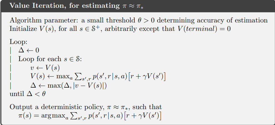
In words, this is the weighted sum of reward plus gamma times the value of the next state weighted over the product of probability of performing this action and the probability of ending up in that state. Our goal is to find the actions in each state that lead to the maximum value for that state. This can be done using the value iteration method, which we will be in using in the next part of the blog where we code this algorithm.
That's all for this part. See you in the next part with some code.
Want to connect?


